数据可视化
在数据科学和分析领域,原始的数字往往难以直接传达其中蕴含的信息和规律。数据可视化就像是一座桥梁,将抽象的数据转化为直观的图形表现,
让我们能够快速洞察数据的趋势、模式和异常。在这一部分,我们将学习如何使用Python强大的可视化工具,
将枯燥的数字变成生动的图表,让数据真正“说话”。
数据可视化的基本理念
数据可视化不仅仅是制作漂亮的图表,更是一门将信息有效传达给观众的艺术与科学。当我们面对大量的数据时,
人类的大脑更擅长处理视觉信息而非数字列表。一个精心设计的图表能够在几秒钟内传达出需要阅读大量文字才能理解的信息。
在现代社会中,数据可视化的应用无处不在。新闻媒体使用图表来解释复杂的社会现象,企业通过仪表板监控业务指标,
科研工作者用图形展示实验结果,教育工作者通过可视化让抽象概念变得具体。无论是简单的柱状图还是复杂的热力图,
每种图表类型都有其独特的表达方式和适用场景。
Python生态系统为数据可视化提供了丰富的工具选择。其中,matplotlib作为最基础也是最灵活的可视化库,
为我们提供了完整的绘图功能;seaborn在matplotlib的基础上,提供了更加优雅的统计图表接口;
而plotly等库则专注于交互式可视化。掌握这些工具,能够让我们针对不同的数据类型和展示需求,
选择最合适的可视化方案。
matplotlib基础架构
matplotlib是Python数据可视化生态系统的基石,几乎所有其他可视化库都建立在它的基础之上。
理解matplotlib的基本架构和使用方式,是掌握Python数据可视化的关键第一步。
matplotlib的导入和基本设置
在开始创建图表之前,我们需要正确导入matplotlib并进行一些基础配置。matplotlib的pyplot模块提供了类似MATLAB的绘图接口,
是最常用的绘图入口。
import matplotlib.pyplot as plt import numpy as np import pandas as pd
# 设置图表风格 plt.style.use( 'default' ) # 也可以选择 'seaborn', 'ggplot' 等风格
# 设置中文字体支持 plt.rcParams[ 'font.sans-serif' ] = [ 'SimHei' , 'Arial Unicode MS' , 'DejaVu Sans' ] plt.rcParams[ 'axes.unicode_minus' ] = False # 解决负号显示问题
# 生成一些示例数据 np.random.seed( 42 ) # 确保结果可重复 dates = pd.date_range( '2024-01-01' , periods = 30 , freq = 'D' ) temperatures = 15 + 10 * np.sin(np.arange( 30 ) * 2 * np.pi / 30 ) + np.random.normal( 0 , 2 , 30 )
print ( "matplotlib环境配置完成" ) print ( f "示例数据:30天的温度记录" ) print ( f "温度范围: { temperatures.min() :.1f } °C 到 { temperatures.max() :.1f } °C" ) 在这个基础配置中,我们不仅导入了必要的库,还解决了中文显示问题。中文字体的设置对于创建面向中文用户的图表至关重要,
因为matplotlib默认不支持中文字符。通过设置字体参数,我们确保了图表中的中文标题、标签和说明都能正确显示。
图表的基本结构理解
matplotlib的图表由多个层次的组件构成,理解这种层次结构有助于我们更好地控制图表的各个方面。
最顶层是Figure,相当于整个画布;在Figure中可以包含一个或多个Axes,每个Axes就是一个具体的绘图区域;
在Axes中,我们可以添加各种图形元素,如线条、文字、图例等。
# 创建一个基本的图表来理解matplotlib的结构 fig, ax = plt.subplots( figsize = ( 10 , 6 ))
# 绘制温度变化曲线 line = ax.plot(dates, temperatures, linewidth = 2 , color = 'steelblue' , label = '日平均温度' )
# 添加图表标题和轴标签 ax.set_title( '2024年1月份气温变化趋势' , fontsize = 16 , fontweight = 'bold' , pad 这个例子展示了matplotlib图表的基本组成要素。Figure对象管理整个图表的大小和布局,
Axes对象负责具体的绘图操作和坐标系管理。通过分别设置标题、坐标轴标签、网格和图例,
我们创建了一个信息完整、外观专业的图表。
图表的保存和输出
创建图表后,我们通常需要将其保存为文件或在不同的环境中显示。matplotlib提供了灵活的输出选项,
支持多种图片格式和显示方式。
# 创建一个更复杂的图表用于保存演示 fig, (ax1, ax2) = plt.subplots( 2 , 1 , figsize = ( 12 , 8 ))
# 上图:温度趋势 ax1.plot(dates, temperatures, 'o-' , linewidth = 2 , markersize = 4 , color = 'crimson' , alpha = 0.8 , label = '实际温度' )
# 添加趋势线 图表的保存功能让我们能够将可视化结果用于报告、演示或网页展示。不同的文件格式有其特定的用途:
PNG格式支持透明背景,适合网页使用;PDF格式是矢量图,可以无损缩放,适合印刷;
SVG格式也是矢量图,适合网页中的交互应用。
Matplotlib 架构可视化模拟器
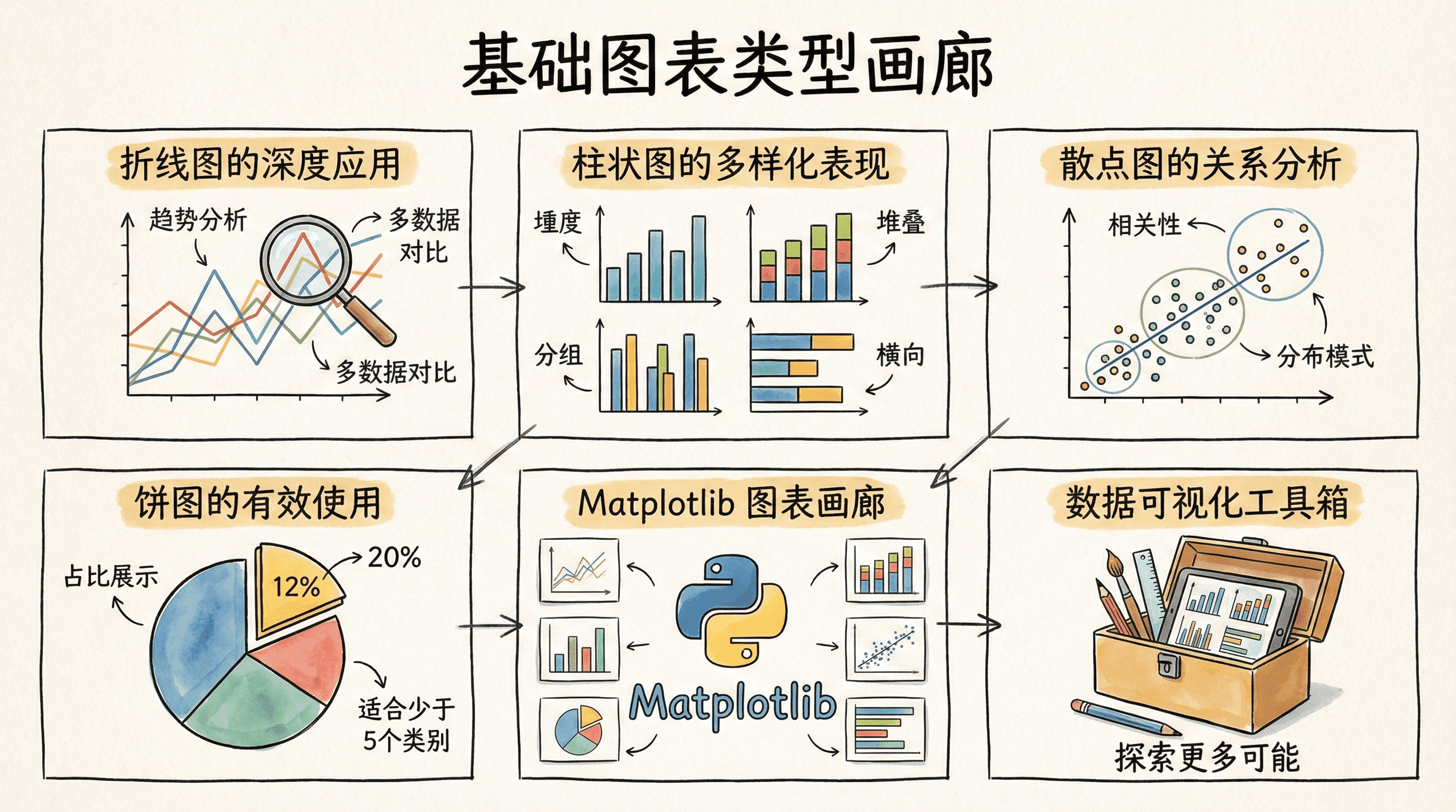
基础图表类型
不同的数据类型和分析目的需要使用不同的图表类型。掌握各种基础图表的特点和适用场景,
是进行有效数据可视化的前提。每种图表类型都有其独特的信息传达方式和视觉效果。
折线图的深度应用
折线图是展示数据随时间或其他连续变量变化趋势的最佳选择。它不仅能显示数据的整体走势,
还能突出变化的速度和波动性。在金融分析、科学研究、业务监控等领域,折线图都是不可或缺的工具。
# 创建多条线的折线图,展示不同城市的气温对比 np.random.seed( 42 ) days = np.arange( 1 , 31 )
# 模拟三个城市的温度数据 beijing_temp = 5 + 8 * np.sin(days * 2 * np.pi / 30 ) + np.random.normal( 0 , 1.5 , 30 ) shanghai_temp = 12 + 6 * np.sin(days 这个例子展示了折线图的高级用法。通过使用不同的标记样式和颜色,我们可以在同一个图表中比较多个数据系列。
添加平均线有助于观众理解数据的整体水平,而网格的使用让数值读取更加精确。
柱状图的多样化表现
柱状图是比较不同类别数据的理想选择。它能够清晰地展示各个类别之间的差异,
并且支持多种样式来适应不同的展示需求。无论是简单的类别比较还是复杂的分组数据,
柱状图都能提供直观的视觉表现。
# 创建一个展示学生成绩分布的柱状图 subjects = [ '语文' , '数学' , '英语' , '物理' , '化学' , '生物' ] class_a_scores = [ 85 , 92 , 78 , 88 , 91 , 86 ] class_b_scores = [ 82 , 89 , 85 , 84 , 87 , 这个柱状图例子展示了如何处理分组数据的可视化。通过并列放置不同组的柱子,
我们可以轻松比较各组在不同类别上的表现。数值标签的添加让观众能够获得精确的数值信息,
而参考线的使用有助于理解数据相对于整体水平的位置。
散点图的关系分析
散点图是探索两个变量之间关系的强大工具。它不仅能显示变量间的相关性,
还能帮助我们识别异常值、聚类模式和非线性关系。在数据分析的初步探索阶段,
散点图往往是第一选择。
# 创建一个分析学习时间与考试成绩关系的散点图 np.random.seed( 42 ) n_students = 120
# 生成学习时间数据(小时/天) study_hours = np.random.normal( 4 , 1.5 , n_students) study_hours = np.clip(study_hours, 1 , 8 ) # 限制在合理范围内
# 生成考试成绩,与学习时间相关但有噪声 base_score = 40 + study_hours * 8 noise = np.random.normal( 0 , 8 , n_students) 散点图的这个例子展示了如何通过可视化探索变量间的关系。通过使用不同颜色表示不同的分类,
添加趋势线显示整体关系,标识异常值突出特殊情况,我们创建了一个信息丰富的分析图表。
统计信息文本框的添加让观众能够快速获得关键的数值指标。
饼图的有效使用
饼图适合展示部分与整体的关系,特别是当我们需要强调某个类别占总体的比例时。
虽然饼图在某些情况下不如柱状图精确,但它在展示构成比例方面具有独特优势。
# 创建一个展示学校预算分配的饼图 budget_categories = [ '教学设备' , '师资培训' , '基础设施' , '学生活动' , '图书采购' , '其他费用' ] budget_amounts = [ 380 , 200 , 150 , 120 , 100 , 50 ] total_budget = sum (budget_amounts)
# 计算百分比 percentages = [amount / total_budget 饼图的例子展示了如何有效地展示预算分配等比例数据。通过使用爆炸效果突出重点,
添加阴影增强立体感,以及创建对比图表展示年度变化,我们创建了既美观又信息丰富的可视化。
Matplotlib 图表画廊
高级图表定制
掌握基础图表类型后,我们需要学习如何深度定制图表的外观和行为,
以满足特定的展示需求和美学要求。高级定制不仅能提升图表的专业度,
还能更好地传达数据背后的信息。
图表样式和主题
matplotlib提供了多种预设样式,同时也支持完全自定义的主题设计。
选择合适的样式可以让图表在不同的使用场景中发挥最佳效果。
# 展示不同样式的效果对比 np.random.seed( 42 ) x = np.linspace( 0 , 10 , 100 ) y1 = np.sin(x) + 0.1 * np.random.randn( 100 ) y2 = np.cos(x) + 0.1 * np.random.randn( 100 )
# 可用的样式列表 available_styles = [ 'default' , 'seaborn-v0_8' , 'ggplot' , 注释和标记的高级应用
在复杂的数据图表中,适当的注释和标记能够引导观众的注意力,
突出关键信息,并提供必要的解释说明。
# 创建一个带有详细注释的股价分析图 np.random.seed( 42 ) dates = pd.date_range( '2024-01-01' , periods = 120 , freq = 'D' )
# 模拟股价数据 price_start = 100 returns = np.random.normal( 0.001 , 0.02 , 120 ) # 日收益率 prices = [price_start] for ret in returns: prices.append(prices[ 多子图布局的艺术
当需要在一个图表中展示多个相关的数据视角时,合理的子图布局设计至关重要。
好的布局不仅能有效利用空间,还能引导观众的阅读顺序和理解逻辑。
# 创建一个综合的数据分析仪表板 np.random.seed( 42 )
# 生成模拟数据 months = [ '1月' , '2月' , '3月' , '4月' , '5月' , '6月' ] revenue = [ 120 , 135 , 150 , 145 , 170 , 185 ] # 营收 cost = [ 80 , 85 这个复杂的多子图例子展示了如何将不同类型的图表组合在一起,
创建一个信息丰富的业务仪表板。通过合理的布局设计和一致的视觉风格,
我们能够在有限的空间内展示多个维度的数据分析结果。
统计图表与seaborn
虽然matplotlib提供了强大的底层绘图功能,但在进行统计分析和数据探索时,
seaborn提供了更加便捷和美观的高级接口。seaborn专门为统计可视化而设计,
能够自动处理许多复杂的统计计算和美化工作。
seaborn的优势与基础使用
seaborn建立在matplotlib之上,但提供了更高层次的抽象和更美观的默认样式。
它特别擅长处理pandas DataFrame,并且内置了许多统计图表类型。
import seaborn as sns import pandas as pd
# 设置seaborn样式 sns.set_style( "whitegrid" ) sns.set_palette( "husl" )
# 创建模拟的学生数据集 np.random.seed( 42 ) n_students = 200
# 生成学生数据 student_data = { 'name' : [ f '学生 { i :03d } ' for i in 高级统计可视化
seaborn的真正威力在于其统计可视化功能。它能够自动计算和展示各种统计指标,
帮助我们深入理解数据的分布特征和变量间的关系。
# 创建高级统计可视化分析 plt.figure( figsize = ( 20 , 15 ))
# 使用subplot_mosaic创建复杂布局 mosaic = """ AABBCC AABBCC DDDEEF DDDEEF GGHHII """
fig, axes = plt.subplot_mosaic(mosaic, figsize = ( 20 , 15 ))
# A. 分布图与核密度估计 sns.histplot( data = df, x = 'total_score' 习题
A. matplotlib
B. seaborn
C. plotly
D. pandas
A. plt.bar()
B. plt.plot()
C. plt.scatter()
D. plt.pie()
A. 展示趋势变化
B. 比较类别大小
C. 显示相关关系
D. 展示分布情况
A. plt.show()
B. plt.display()
C. plt.print()
D. plt.view()
A. fig, ax = plt.subplots()
B. plt.figure()
C. plt.subplot()
D. 以上都可以
6. matplotlib基本绘图
编写一个程序,绘制正弦函数的折线图,并添加标题和坐标轴标签。
import matplotlib.pyplot as plt import numpy as np
# 生成数据 x = np.linspace( 0 , 10 , 100 ) y = np.sin(x)
# 绘制折线图 plt.plot(x, y) plt.title( '正弦函数图' ) plt.xlabel( 'x' ) plt.ylabel( 'sin(x)' ) plt.show() 说明:
np.linspace(0, 10, 100)生成0到10之间的100个等间距数值np.sin(x)计算正弦值plt.plot(x, y)绘制折线图 7. 柱状图绘制
编写一个程序,绘制类别数据的柱状图。
import matplotlib.pyplot as plt
categories = [ 'A' , 'B' , 'C' , 'D' ] values = [ 23 , 45 , 56 , 78 ]
# 绘制柱状图 plt.bar(categories, values) plt.title( '类别数据对比' ) plt.xlabel( '类别' ) plt.ylabel( '数值' ) plt.show() 8. 散点图绘制
编写一个程序,绘制散点图展示两个变量之间的关系。
import matplotlib.pyplot as plt import numpy as np
# 生成模拟数据 np.random.seed( 42 ) height = np.random.normal( 170 , 10 , 100 ) # 身高数据 weight = height * 0.5 + np.random.normal( 0 , 5 , 100 ) # 体重数据(与身高相关)
# 绘制散点图 plt.scatter(height, weight, alpha =
20
)
ax.set_xlabel( '日期' , fontsize = 12 )
ax.set_ylabel( '温度 (°C)' , fontsize = 12 )
# 设置坐标轴格式
ax.tick_params( axis = 'x' , rotation = 45 ) # 旋转x轴标签
ax.grid( True , alpha = 0.3 ) # 添加网格
# 添加图例
ax.legend( loc = 'upper right' )
# 调整布局以避免标签被截断
plt.tight_layout()
# 显示图表
plt.show()
print ( "基础图表创建完成" )
print ( "图表包含:标题、坐标轴标签、网格、图例等基本元素" )
z
=
np.polyfit(
range
(
len
(temperatures)), temperatures,
1
)
trend_line = np.poly1d(z)
ax1.plot(dates, trend_line( range ( len (temperatures))), '--' ,
color = 'darkblue' , linewidth = 2 , label = '趋势线' )
ax1.set_title( '气温变化趋势分析' , fontsize = 14 , fontweight = 'bold' )
ax1.set_ylabel( '温度 (°C)' , fontsize = 12 )
ax1.legend()
ax1.grid( True , alpha = 0.3 )
# 下图:温度分布直方图
ax2.hist(temperatures, bins = 15 , color = 'lightcoral' , alpha = 0.7 ,
edgecolor = 'black' , linewidth = 1 )
ax2.set_title( '气温分布直方图' , fontsize = 14 , fontweight = 'bold' )
ax2.set_xlabel( '温度 (°C)' , fontsize = 12 )
ax2.set_ylabel( '频次' , fontsize = 12 )
ax2.grid( True , alpha = 0.3 )
# 调整子图间距
plt.tight_layout()
# 保存图表为不同格式
plt.savefig( 'temperature_analysis.png' , dpi = 300 , bbox_inches = 'tight' )
plt.savefig( 'temperature_analysis.pdf' , bbox_inches = 'tight' )
plt.show()
print ( "图表已保存为PNG和PDF格式" )
print ( "PNG格式适合网页显示,PDF格式适合印刷和学术用途" )
*
2
*
np.pi
/
30
)
+
np.random.normal(
0
,
1.2
,
30
)
guangzhou_temp = 18 + 4 * np.sin(days * 2 * np.pi / 30 ) + np.random.normal( 0 , 1 , 30 )
# 创建折线图
plt.figure( figsize = ( 12 , 8 ))
# 绘制三条线,使用不同的样式
plt.plot(days, beijing_temp, 'o-' , linewidth = 2.5 , markersize = 5 ,
color = 'royalblue' , label = '北京' , alpha = 0.8 )
plt.plot(days, shanghai_temp, 's-' , linewidth = 2.5 , markersize = 4 ,
color = 'forestgreen' , label = '上海' , alpha = 0.8 )
plt.plot(days, guangzhou_temp, '^-' , linewidth = 2.5 , markersize = 4 ,
color = 'orangered' , label = '广州' , alpha = 0.8 )
# 添加平均温度线
overall_mean = np.mean([beijing_temp.mean(), shanghai_temp.mean(), guangzhou_temp.mean()])
plt.axhline( y = overall_mean, color = 'gray' , linestyle = '--' , linewidth = 2 ,
alpha = 0.7 , label = f '三城市平均温度 ( { overall_mean :.1f } °C)' )
# 图表美化
plt.title( '三大城市一月份气温对比分析' , fontsize = 16 , fontweight = 'bold' , pad = 20 )
plt.xlabel( '日期 (1月)' , fontsize = 12 )
plt.ylabel( '气温 (°C)' , fontsize = 12 )
# 自定义网格
plt.grid( True , linestyle = '-' , alpha = 0.2 )
plt.grid( True , linestyle = ':' , alpha = 0.5 , which = 'minor' )
# 图例设置
plt.legend( loc = 'upper left' , frameon = True , fancybox = True , shadow = True )
# 设置坐标轴范围
plt.xlim( 0 , 31 )
plt.ylim( min (beijing_temp.min(), shanghai_temp.min(), guangzhou_temp.min()) - 2 ,
max (beijing_temp.max(), shanghai_temp.max(), guangzhou_temp.max()) + 2 )
plt.tight_layout()
plt.show()
print ( "多线折线图展示了三个城市的气温变化对比" )
print ( f "北京平均气温: { beijing_temp.mean() :.1f } °C" )
print ( f "上海平均气温: { shanghai_temp.mean() :.1f } °C" )
print ( f "广州平均气温: { guangzhou_temp.mean() :.1f } °C" )
90
]
class_c_scores = [ 88 , 85 , 82 , 91 , 89 , 83 ]
# 设置柱状图的位置
x = np.arange( len (subjects))
width = 0.25
# 创建图表
fig, ax = plt.subplots( figsize = ( 12 , 8 ))
# 绘制三组柱状图
bars1 = ax.bar(x - width, class_a_scores, width, label = 'A班' ,
color = 'lightcoral' , alpha = 0.8 , edgecolor = 'darkred' , linewidth = 1 )
bars2 = ax.bar(x, class_b_scores, width, label = 'B班' ,
color = 'lightblue' , alpha = 0.8 , edgecolor = 'darkblue' , linewidth = 1 )
bars3 = ax.bar(x + width, class_c_scores, width, label = 'C班' ,
color = 'lightgreen' , alpha = 0.8 , edgecolor = 'darkgreen' , linewidth = 1 )
# 在柱状图上添加数值标签
def add_value_labels (bars):
"""在柱状图上添加数值标签"""
for bar in bars:
height = bar.get_height()
ax.annotate( f ' { height } ' ,
xy = (bar.get_x() + bar.get_width() / 2 , height),
xytext = ( 0 , 3 ), # 3 points vertical offset
textcoords = "offset points" ,
ha = 'center' , va = 'bottom' ,
fontsize = 9 , fontweight = 'bold' )
add_value_labels(bars1)
add_value_labels(bars2)
add_value_labels(bars3)
# 图表美化
ax.set_title( '三个班级各科成绩对比分析' , fontsize = 16 , fontweight = 'bold' , pad = 20 )
ax.set_xlabel( '科目' , fontsize = 12 )
ax.set_ylabel( '平均成绩' , fontsize = 12 )
ax.set_xticks(x)
ax.set_xticklabels(subjects)
# 添加平均分参考线
overall_average = np.mean([class_a_scores, class_b_scores, class_c_scores])
ax.axhline( y = overall_average, color = 'red' , linestyle = '--' , linewidth = 2 ,
alpha = 0.7 , label = f '总体平均分 ( { overall_average :.1f } )' )
# 图例和网格
ax.legend( loc = 'upper right' )
ax.grid( True , axis = 'y' , alpha = 0.3 )
# 设置y轴范围,留出空间显示标签
ax.set_ylim( 70 , 100 )
plt.tight_layout()
plt.show()
# 计算并显示统计信息
print ( "各班级平均成绩统计:" )
print ( f "A班总平均: { np.mean(class_a_scores) :.1f } 分" )
print ( f "B班总平均: { np.mean(class_b_scores) :.1f } 分" )
print ( f "C班总平均: { np.mean(class_c_scores) :.1f } 分" )
# 找出各科最高分的班级
best_performers = []
for i, subject in enumerate (subjects):
scores = [class_a_scores[i], class_b_scores[i], class_c_scores[i]]
best_class = [ 'A班' , 'B班' , 'C班' ][np.argmax(scores)]
best_performers.append((subject, best_class, max (scores)))
print ( " \n 各科最佳表现:" )
for subject, class_name, score in best_performers:
print ( f " { subject } : { class_name } ( { score } 分)" )
exam_scores = base_score + noise
exam_scores = np.clip(exam_scores, 0 , 100 ) # 限制在0-100分
# 创建不同学生类型的标识
student_types = np.random.choice([ '文科生' , '理科生' , '艺术生' ], n_students,
p = [ 0.4 , 0.4 , 0.2 ])
# 为不同类型学生设置颜色
type_colors = { '文科生' : 'lightcoral' , '理科生' : 'lightblue' , '艺术生' : 'lightgreen' }
colors = [type_colors[t] for t in student_types]
# 创建散点图
plt.figure( figsize = ( 12 , 8 ))
# 绘制不同类型学生的散点
for student_type in [ '文科生' , '理科生' , '艺术生' ]:
mask = student_types == student_type
plt.scatter(study_hours[mask], exam_scores[mask],
c = type_colors[student_type], alpha = 0.6 , s = 60 ,
edgecolors = 'black' , linewidth = 0.5 , label = student_type)
# 添加趋势线
z = np.polyfit(study_hours, exam_scores, 1 )
trend_line = np.poly1d(z)
x_trend = np.linspace(study_hours.min(), study_hours.max(), 100 )
plt.plot(x_trend, trend_line(x_trend), 'red' , linewidth = 3 ,
linestyle = '--' , alpha = 0.8 , label = f '趋势线 (R²= { np.corrcoef(study_hours, exam_scores)[ 0 , 1 ] ** 2 :.3f } )' )
# 标识异常值(成绩特别高或特别低的学生)
residuals = exam_scores - trend_line(study_hours)
outliers = np.abs(residuals) > 2 * np.std(residuals)
if outliers.any():
plt.scatter(study_hours[outliers], exam_scores[outliers],
c = 'red' , s = 100 , marker = 'x' , linewidth = 3 ,
label = f '异常值 ( { outliers.sum() } 个)' )
# 图表美化
plt.title( '学习时间与考试成绩关系分析' , fontsize = 16 , fontweight = 'bold' , pad = 20 )
plt.xlabel( '日均学习时间 (小时)' , fontsize = 12 )
plt.ylabel( '考试成绩 (分)' , fontsize = 12 )
# 添加网格和图例
plt.grid( True , alpha = 0.3 )
plt.legend( loc = 'lower right' )
# 添加统计信息文本框
correlation = np.corrcoef(study_hours, exam_scores)[ 0 , 1 ]
stats_text = f '相关系数: { correlation :.3f }\n 样本数量: { n_students }\n 平均学习时间:
{ study_hours.mean() :.1f } 小时 \n 平均成绩: { exam_scores.mean() :.1f } 分'
plt.text( 0.02 , 0.98 , stats_text, transform = plt.gca().transAxes,
verticalalignment = 'top' , bbox = dict ( boxstyle = 'round' , facecolor = 'wheat' , alpha = 0.8 ))
plt.tight_layout()
plt.show()
# 详细统计分析
print ( "学习时间与成绩关系分析结果:" )
print ( f "相关系数: { correlation :.3f } " )
print ( f "相关强度: { '强' if abs (correlation) > 0.7 else '中等' if abs (correlation) > 0.4 else '弱' } " )
# 不同类型学生的统计
print ( " \n 不同类型学生表现:" )
for student_type in [ '文科生' , '理科生' , '艺术生' ]:
mask = student_types == student_type
avg_hours = study_hours[mask].mean()
avg_score = exam_scores[mask].mean()
print ( f " { student_type } :平均学习 { avg_hours :.1f } 小时,平均成绩 { avg_score :.1f } 分" )
*
100
for
amount
in
budget_amounts]
# 设置颜色方案
colors = [ '#FF6B6B' , '#4ECDC4' , '#45B7D1' , '#96CEB4' , '#FFEAA7' , '#DDA0DD' ]
# 突出显示最大的类别
explode = [ 0.1 if amount == max (budget_amounts) else 0 for amount in budget_amounts]
# 创建饼图
plt.figure( figsize = ( 12 , 8 ))
# 绘制饼图
wedges, texts, autotexts = plt.pie(budget_amounts, labels = budget_categories,
autopct = ' %1.1f%% ' , startangle = 90 ,
colors = colors, explode = explode,
shadow = True , pctdistance = 0.85 )
# 美化文本
for autotext in autotexts:
autotext.set_color( 'white' )
autotext.set_fontweight( 'bold' )
autotext.set_fontsize( 10 )
for text in texts:
text.set_fontsize( 11 )
text.set_fontweight( 'bold' )
# 添加标题
plt.title( '学校年度预算分配情况 \n (总预算:¥ {} 万元)' .format(total_budget),
fontsize = 16 , fontweight = 'bold' , pad = 20 )
# 添加图例,显示具体金额
legend_labels = [ f ' { cat } :¥ { amount } 万元' for cat, amount in zip (budget_categories, budget_amounts)]
plt.legend(wedges, legend_labels, title = "预算详情" , loc = "center left" ,
bbox_to_anchor = ( 1 , 0 , 0.5 , 1 ))
# 保证饼图是圆形
plt.axis( 'equal' )
plt.tight_layout()
plt.show()
# 创建对比环形图显示预算变化
fig, (ax1, ax2) = plt.subplots( 1 , 2 , figsize = ( 16 , 8 ))
# 今年预算
wedges1, texts1, autotexts1 = ax1.pie(budget_amounts, labels = budget_categories,
autopct = ' %1.1f%% ' , startangle = 90 ,
colors = colors, pctdistance = 0.85 ,
wedgeprops = dict ( width = 0.5 ))
ax1.set_title( '2024年预算分配' , fontsize = 14 , fontweight = 'bold' )
# 去年预算(模拟数据)
last_year_amounts = [ 350 , 180 , 180 , 100 , 120 , 70 ]
wedges2, texts2, autotexts2 = ax2.pie(last_year_amounts, labels = budget_categories,
autopct = ' %1.1f%% ' , startangle = 90 ,
colors = colors, pctdistance = 0.85 ,
wedgeprops = dict ( width = 0.5 ))
ax2.set_title( '2023年预算分配' , fontsize = 14 , fontweight = 'bold' )
# 美化文本
for autotexts in [autotexts1, autotexts2]:
for autotext in autotexts:
autotext.set_color( 'white' )
autotext.set_fontweight( 'bold' )
autotext.set_fontsize( 9 )
plt.tight_layout()
plt.show()
# 预算变化分析
print ( "预算分配分析:" )
print ( f "总预算: { total_budget } 万元" )
print ( f "最大支出项目: { budget_categories[budget_amounts.index( max (budget_amounts))] } ( {max (budget_amounts) } 万元)" )
print ( " \n 各项目占比:" )
for cat, amount, pct in zip (budget_categories, budget_amounts, percentages):
print ( f " { cat } : { amount } 万元 ( { pct :.1f } %)" )
# 与去年对比
print ( " \n 与去年预算对比:" )
for i, (cat, this_year, last_year) in enumerate ( zip (budget_categories, budget_amounts, last_year_amounts)):
change = this_year - last_year
change_pct = (change / last_year) * 100 if last_year > 0 else 0
print ( f " { cat } : { '增加' if change > 0 else '减少' } ¥ {abs (change) } 万元 ( { change_pct :+.1f } %)" )
'classic'
]
fig, axes = plt.subplots( 2 , 2 , figsize = ( 16 , 12 ))
axes = axes.ravel()
for i, style in enumerate (available_styles):
plt.style.use(style)
# 在子图中绘制
ax = axes[i]
ax.plot(x, y1, label = 'sin(x)' , linewidth = 2 )
ax.plot(x, y2, label = 'cos(x)' , linewidth = 2 )
ax.set_title( f ' { style } 样式' , fontsize = 12 , fontweight = 'bold' )
ax.legend()
ax.grid( True , alpha = 0.3 )
plt.tight_layout()
plt.show()
# 重置为默认样式
plt.style.use( 'default' )
# 创建自定义样式的图表
plt.figure( figsize = ( 12 , 8 ))
# 自定义颜色方案
custom_colors = [ '#2E8B57' , '#4169E1' , '#DC143C' , '#FF8C00' , '#9932CC' ]
# 创建多个数据系列
data_series = []
labels = [ '产品A' , '产品B' , '产品C' , '产品D' , '产品E' ]
months = [ '1月' , '2月' , '3月' , '4月' , '5月' , '6月' ]
for i in range ( 5 ):
# 生成模拟销售数据
trend = np.linspace( 100 + i * 20 , 200 + i * 30 , 6 )
noise = np.random.normal( 0 , 10 , 6 )
sales = trend + noise
data_series.append(sales)
# 绘制线图
for i, (sales, label, color) in enumerate ( zip (data_series, labels, custom_colors)):
plt.plot(months, sales, 'o-' , linewidth = 3 , markersize = 8 ,
color = color, label = label, alpha = 0.8 ,
markeredgecolor = 'white' , markeredgewidth = 2 )
# 高级定制
plt.title( '各产品月度销售趋势' , fontsize = 18 , fontweight = 'bold' ,
color = 'darkslategray' , pad = 25 )
plt.xlabel( '月份' , fontsize = 14 , fontweight = 'bold' , color = 'darkslategray' )
plt.ylabel( '销售额 (万元)' , fontsize = 14 , fontweight = 'bold' , color = 'darkslategray' )
# 自定义网格
plt.grid( True , linestyle = '--' , alpha = 0.7 , color = 'lightgray' )
# 设置背景颜色
plt.gca().set_facecolor( '#FAFAFA' )
# 自定义图例
plt.legend( frameon = True , fancybox = True , shadow = True ,
framealpha = 0.9 , facecolor = 'white' , edgecolor = 'gray' ,
loc = 'upper left' )
# 设置坐标轴样式
plt.gca().spines[ 'top' ].set_visible( False )
plt.gca().spines[ 'right' ].set_visible( False )
plt.gca().spines[ 'left' ].set_color( 'darkgray' )
plt.gca().spines[ 'bottom' ].set_color( 'darkgray' )
# 调整刻度标签
plt.xticks( fontsize = 12 , color = 'darkslategray' )
plt.yticks( fontsize = 12 , color = 'darkslategray' )
plt.tight_layout()
plt.show()
print ( "图表样式定制演示完成" )
print ( "展示了从预设样式到完全自定义的各种可能性" )
-
1
]
*
(
1
+
ret))
prices = np.array(prices[ 1 :]) # 去掉初始值
# 计算移动平均线
ma_20 = pd.Series(prices).rolling( window = 20 ).mean()
ma_50 = pd.Series(prices).rolling( window = 50 ).mean()
# 找出重要的点位
max_price_idx = np.argmax(prices)
min_price_idx = np.argmin(prices)
latest_price = prices[ - 1 ]
# 创建图表
plt.figure( figsize = ( 15 , 10 ))
# 绘制股价和移动平均线
plt.plot(dates, prices, linewidth = 2 , color = 'darkblue' , label = '股价' , alpha = 0.8 )
plt.plot(dates, ma_20, linewidth = 2 , color = 'orange' , label = '20日移动平均' , alpha = 0.7 )
plt.plot(dates, ma_50, linewidth = 2 , color = 'red' , label = '50日移动平均' , alpha = 0.7 )
# 标记重要点位
plt.scatter(dates[max_price_idx], prices[max_price_idx],
color = 'red' , s = 100 , zorder = 5 , marker = '^' )
plt.scatter(dates[min_price_idx], prices[min_price_idx],
color = 'green' , s = 100 , zorder = 5 , marker = 'v' )
# 添加详细注释
# 最高点注释
plt.annotate( f '最高价: ¥ { prices[max_price_idx] :.2f }\n{ dates[max_price_idx].strftime( "%Y-%m- %d " ) } ' ,
xy = (dates[max_price_idx], prices[max_price_idx]),
xytext = ( 20 , 20 ), textcoords = 'offset points' ,
bbox = dict ( boxstyle = 'round,pad=0.5' , fc = 'red' , alpha = 0.7 ),
arrowprops = dict ( arrowstyle = '->' , connectionstyle = 'arc3,rad=0' ),
fontsize = 10 , color = 'white' , fontweight = 'bold' )
# 最低点注释
plt.annotate( f '最低价: ¥ { prices[min_price_idx] :.2f }\n{ dates[min_price_idx].strftime( "%Y-%m- %d " ) } ' ,
xy = (dates[min_price_idx], prices[min_price_idx]),
xytext = ( 20 , - 30 ), textcoords = 'offset points' ,
bbox = dict ( boxstyle = 'round,pad=0.5' , fc = 'green' , alpha = 0.7 ),
arrowprops = dict ( arrowstyle = '->' , connectionstyle = 'arc3,rad=0' ),
fontsize = 10 , color = 'white' , fontweight = 'bold' )
# 添加当前价格线
plt.axhline( y = latest_price, color = 'purple' , linestyle = ':' , linewidth = 2 , alpha = 0.7 )
plt.text(dates[ 10 ], latest_price + 1 , f '当前价格: ¥ { latest_price :.2f } ' ,
fontsize = 11 , fontweight = 'bold' , color = 'purple' ,
bbox = dict ( boxstyle = 'round,pad=0.3' , facecolor = 'lavender' , alpha = 0.8 ))
# 添加区间填充
bullish_mask = prices > ma_20
plt.fill_between(dates, prices.min(), prices.max(),
where = bullish_mask, alpha = 0.1 , color = 'green' ,
label = '价格高于20日均线区间' )
# 标题和标签
plt.title( 'XYZ科技股股价走势分析 \n (2024年1-4月)' ,
fontsize = 16 , fontweight = 'bold' , pad = 20 )
plt.xlabel( '日期' , fontsize = 12 , fontweight = 'bold' )
plt.ylabel( '股价 (¥)' , fontsize = 12 , fontweight = 'bold' )
# 自定义图例
plt.legend( loc = 'upper left' , frameon = True , fancybox = True ,
shadow = True , framealpha = 0.9 )
# 网格和格式
plt.grid( True , alpha = 0.3 )
plt.xticks( rotation = 45 )
# 添加统计信息框
stats_text = f '''统计信息:
期初价格: ¥ { prices[ 0 ] :.2f }
期末价格: ¥ { prices[ - 1 ] :.2f }
总收益率: { ((prices[ - 1 ] / prices[ 0 ]) - 1 ) * 100 :+.1f } %
最大回撤: { ((prices.min() / prices.max()) - 1 ) * 100 :.1f } %
波动率: { np.std(returns) * np.sqrt( 252 ) * 100 :.1f } %'''
plt.text( 0.02 , 0.98 , stats_text, transform = plt.gca().transAxes,
verticalalignment = 'top' , fontsize = 10 ,
bbox = dict ( boxstyle = 'round' , facecolor = 'wheat' , alpha = 0.8 ))
plt.tight_layout()
plt.show()
print ( "高级注释图表演示完成" )
print ( "展示了如何使用注释、标记和填充区域来增强图表的信息传达能力" )
,
95
,
90
,
105
,
115
]
# 成本
profit = [r - c for r, c in zip (revenue, cost)] # 利润
# 客户满意度数据
satisfaction_categories = [ '非常满意' , '满意' , '一般' , '不满意' , '非常不满意' ]
satisfaction_counts = [ 45 , 32 , 15 , 6 , 2 ]
# 产品销量数据
products = [ '产品A' , '产品B' , '产品C' , '产品D' , '产品E' ]
q1_sales = [ 25 , 20 , 30 , 15 , 10 ]
q2_sales = [ 30 , 25 , 35 , 18 , 12 ]
# 创建复杂的子图布局
fig = plt.figure( figsize = ( 16 , 12 ))
gs = fig.add_gridspec( 3 , 3 , height_ratios = [ 1 , 1 , 1 ], width_ratios = [ 2 , 1 , 1 ])
# 1. 主图:营收和利润趋势 (占据前两列的第一行)
ax1 = fig.add_subplot(gs[ 0 , : 2 ])
x_pos = np.arange( len (months))
# 双y轴图表
ax1_twin = ax1.twinx()
# 绘制柱状图(营收和成本)
bars1 = ax1.bar(x_pos - 0.2 , revenue, 0.4 , label = '营收' , color = 'steelblue' , alpha = 0.8 )
bars2 = ax1.bar(x_pos + 0.2 , cost, 0.4 , label = '成本' , color = 'lightcoral' , alpha = 0.8 )
# 绘制利润折线
line = ax1_twin.plot(x_pos, profit, 'go-' , linewidth = 3 , markersize = 8 ,
label = '利润' , color = 'forestgreen' )
# 设置第一个图的样式
ax1.set_title( '财务数据综合分析' , fontsize = 14 , fontweight = 'bold' , pad = 15 )
ax1.set_xlabel( '月份' , fontsize = 11 )
ax1.set_ylabel( '营收/成本 (万元)' , fontsize = 11 , color = 'steelblue' )
ax1_twin.set_ylabel( '利润 (万元)' , fontsize = 11 , color = 'forestgreen' )
ax1.set_xticks(x_pos)
ax1.set_xticklabels(months)
ax1.legend( loc = 'upper left' )
ax1_twin.legend( loc = 'upper right' )
ax1.grid( True , alpha = 0.3 )
# 2. 客户满意度饼图 (第一行第三列)
ax2 = fig.add_subplot(gs[ 0 , 2 ])
colors_pie = [ '#2ecc71' , '#3498db' , '#f39c12' , '#e74c3c' , '#9b59b6' ]
wedges, texts, autotexts = ax2.pie(satisfaction_counts, labels = satisfaction_categories,
autopct = ' %1.1f%% ' , colors = colors_pie,
startangle = 90 , textprops = { 'fontsize' : 8 })
ax2.set_title( '客户满意度分布' , fontsize = 12 , fontweight = 'bold' )
# 3. 产品销量对比图 (第二行第一列)
ax3 = fig.add_subplot(gs[ 1 , 0 ])
x_products = np.arange( len (products))
width = 0.35
bars3 = ax3.bar(x_products - width / 2 , q1_sales, width, label = 'Q1' ,
color = 'lightblue' , alpha = 0.8 )
bars4 = ax3.bar(x_products + width / 2 , q2_sales, width, label = 'Q2' ,
color = 'darkblue' , alpha = 0.8 )
ax3.set_title( '产品销量对比 (Q1 vs Q2)' , fontsize = 12 , fontweight = 'bold' )
ax3.set_xlabel( '产品' )
ax3.set_ylabel( '销量 (万件)' )
ax3.set_xticks(x_products)
ax3.set_xticklabels(products)
ax3.legend()
ax3.grid( True , alpha = 0.3 )
# 4. 增长率分析 (第二行第二列)
ax4 = fig.add_subplot(gs[ 1 , 1 ])
growth_rates = [(q2 - q1) / q1 * 100 for q1, q2 in zip (q1_sales, q2_sales)]
colors_growth = [ 'green' if x > 0 else 'red' for x in growth_rates]
bars5 = ax4.barh(products, growth_rates, color = colors_growth, alpha = 0.7 )
ax4.set_title( 'Q2增长率' , fontsize = 12 , fontweight = 'bold' )
ax4.set_xlabel( '增长率 (%)' )
ax4.axvline( x = 0 , color = 'black' , linestyle = '-' , linewidth = 0.5 )
ax4.grid( True , alpha = 0.3 )
# 5. 月度利润率趋势 (第二行第三列)
ax5 = fig.add_subplot(gs[ 1 , 2 ])
profit_margin = [p / r * 100 for p, r in zip (profit, revenue)]
ax5.plot(months, profit_margin, 'o-' , linewidth = 2 , markersize = 6 ,
color = 'purple' , alpha = 0.8 )
ax5.set_title( '利润率趋势' , fontsize = 12 , fontweight = 'bold' )
ax5.set_ylabel( '利润率 (%)' )
ax5.tick_params( axis = 'x' , rotation = 45 )
ax5.grid( True , alpha = 0.3 )
# 6. 关键指标汇总 (第三行,跨越所有列)
ax6 = fig.add_subplot(gs[ 2 , :])
ax6.axis( 'off' ) # 关闭坐标轴
# 创建指标表格
kpi_data = [
[ '总营收' , f ' {sum (revenue) :.0f } 万元' , '同比增长' , '+15.2%' ],
[ '总成本' , f ' {sum (cost) :.0f } 万元' , '成本控制' , '良好' ],
[ '总利润' , f ' {sum (profit) :.0f } 万元' , '利润率' , f ' {sum (profit) / sum (revenue) * 100 :.1f } %' ],
[ '客户满意度' , '87.5%' , '增长最快产品' , '产品C' ]
]
# 绘制表格
table = ax6.table( cellText = kpi_data,
colLabels = [ '指标' , '数值' , '指标' , '数值' ],
cellLoc = 'center' ,
loc = 'center' ,
colWidths = [ 0.2 , 0.2 , 0.2 , 0.2 ])
table.auto_set_font_size( False )
table.set_fontsize( 11 )
table.scale( 1 , 2 )
# 设置表格样式
for i in range ( len (kpi_data) + 1 ):
for j in range ( 4 ):
cell = table[(i, j)]
if i == 0 : # 表头
cell.set_facecolor( '#4CAF50' )
cell.set_text_props( weight = 'bold' , color = 'white' )
else :
if j % 2 == 0 :
cell.set_facecolor( '#E8F5E8' )
else :
cell.set_facecolor( '#F0F8FF' )
ax6.set_title( '关键业务指标汇总' , fontsize = 14 , fontweight = 'bold' , pad = 20 )
# 调整整体布局
plt.tight_layout()
plt.show()
print ( "多子图仪表板演示完成" )
print ( "展示了如何使用复杂的子图布局创建综合性的数据分析仪表板" )
range
(
1
, n_students
+
1
)],
'gender' : np.random.choice([ '男' , '女' ], n_students, p = [ 0.52 , 0.48 ]),
'grade' : np.random.choice([ '高一' , '高二' , '高三' ], n_students, p = [ 0.35 , 0.35 , 0.3 ]),
'math_score' : np.random.normal( 75 , 15 , n_students),
'english_score' : np.random.normal( 72 , 12 , n_students),
'physics_score' : np.random.normal( 68 , 18 , n_students),
'study_hours' : np.random.gamma( 2 , 2 , n_students),
'family_income' : np.random.lognormal( 10.5 , 0.8 , n_students)
}
# 确保分数在合理范围内
for subject in [ 'math_score' , 'english_score' , 'physics_score' ]:
student_data[subject] = np.clip(student_data[subject], 0 , 100 )
student_data[ 'study_hours' ] = np.clip(student_data[ 'study_hours' ], 1 , 12 )
student_data[ 'family_income' ] = np.clip(student_data[ 'family_income' ], 20000 , 200000 )
# 创建DataFrame
df = pd.DataFrame(student_data)
# 添加总分和排名
df[ 'total_score' ] = df[[ 'math_score' , 'english_score' , 'physics_score' ]].sum( axis = 1 )
df[ 'rank' ] = df[ 'total_score' ].rank( method = 'min' , ascending = False ).astype( int )
print ( "学生数据集创建完成" )
print ( f "数据集包含 {len (df) } 名学生的信息" )
print ( " \n 数据概览:" )
print (df.describe())
# 创建seaborn风格的综合分析图
fig, axes = plt.subplots( 2 , 3 , figsize = ( 18 , 12 ))
# 1. 成绩分布的小提琴图
ax1 = axes[ 0 , 0 ]
score_columns = [ 'math_score' , 'english_score' , 'physics_score' ]
score_data = df[score_columns].melt( var_name = '科目' , value_name = '成绩' )
score_data[ '科目' ] = score_data[ '科目' ].map({
'math_score' : '数学' ,
'english_score' : '英语' ,
'physics_score' : '物理'
})
sns.violinplot( data = score_data, x = '科目' , y = '成绩' , ax = ax1)
ax1.set_title( '各科成绩分布情况' , fontsize = 14 , fontweight = 'bold' )
ax1.set_ylabel( '成绩' )
# 2. 性别与成绩的箱线图
ax2 = axes[ 0 , 1 ]
sns.boxplot( data = score_data, x = '科目' , y = '成绩' ,
hue = df[ 'gender' ].repeat( 3 ).reset_index( drop = True ), ax = ax2)
ax2.set_title( '不同性别各科成绩对比' , fontsize = 14 , fontweight = 'bold' )
ax2.legend( title = '性别' )
# 3. 学习时间与总分的散点图
ax3 = axes[ 0 , 2 ]
sns.scatterplot( data = df, x = 'study_hours' , y = 'total_score' ,
hue = 'grade' , size = 'family_income' ,
sizes = ( 50 , 200 ), alpha = 0.7 , ax = ax3)
ax3.set_title( '学习时间与总分关系' , fontsize = 14 , fontweight = 'bold' )
ax3.set_xlabel( '日均学习时间 (小时)' )
ax3.set_ylabel( '总分' )
# 4. 年级分布的条形图
ax4 = axes[ 1 , 0 ]
grade_counts = df[ 'grade' ].value_counts()
sns.barplot( x = grade_counts.index, y = grade_counts.values, ax = ax4)
ax4.set_title( '年级分布情况' , fontsize = 14 , fontweight = 'bold' )
ax4.set_xlabel( '年级' )
ax4.set_ylabel( '学生数量' )
# 在柱状图上添加数值标签
for i, v in enumerate (grade_counts.values):
ax4.text(i, v + 1 , str (v), ha = 'center' , va = 'bottom' , fontweight = 'bold' )
# 5. 科目间相关性热力图
ax5 = axes[ 1 , 1 ]
correlation_matrix = df[[ 'math_score' , 'english_score' , 'physics_score' , 'study_hours' ]].corr()
correlation_matrix.columns = [ '数学' , '英语' , '物理' , '学习时间' ]
correlation_matrix.index = [ '数学' , '英语' , '物理' , '学习时间' ]
sns.heatmap(correlation_matrix, annot = True , cmap = 'coolwarm' , center = 0 ,
square = True , ax = ax5, fmt = '.2f' )
ax5.set_title( '科目间相关性分析' , fontsize = 14 , fontweight = 'bold' )
# 6. 家庭收入分布的直方图
ax6 = axes[ 1 , 2 ]
sns.histplot( data = df, x = 'family_income' , bins = 20 , kde = True , ax = ax6)
ax6.set_title( '家庭收入分布' , fontsize = 14 , fontweight = 'bold' )
ax6.set_xlabel( '家庭年收入 (元)' )
ax6.set_ylabel( '频次' )
# 格式化x轴标签
ax6.xaxis.set_major_formatter(plt.FuncFormatter( lambda x, p: f ' { x / 10000 :.0f } 万' ))
plt.tight_layout()
plt.show()
# 统计分析
print ( " \n 详细统计分析:" )
# 各年级平均成绩
print ( "各年级平均总分:" )
grade_avg = df.groupby( 'grade' )[ 'total_score' ].mean().sort_values( ascending = False )
for grade, avg_score in grade_avg.items():
print ( f " { grade } : { avg_score :.1f } 分" )
# 性别差异分析
print ( " \n 性别成绩差异:" )
gender_stats = df.groupby( 'gender' )[[ 'math_score' , 'english_score' , 'physics_score' ]].mean()
for gender in [ '男' , '女' ]:
print ( f " { gender } 生平均成绩:" )
print ( f " 数学: { gender_stats.loc[gender, 'math_score' ] :.1f } 分" )
print ( f " 英语: { gender_stats.loc[gender, 'english_score' ] :.1f } 分" )
print ( f " 物理: { gender_stats.loc[gender, 'physics_score' ] :.1f } 分" )
# 学习时间与成绩的相关性
correlation = df[ 'study_hours' ].corr(df[ 'total_score' ])
print ( f " \n 学习时间与总分相关系数: { correlation :.3f } " )
,
hue
=
'grade'
,
element = 'step' , stat = 'density' , common_norm = False ,
alpha = 0.7 , ax = axes[ 'A' ])
axes[ 'A' ].set_title( '各年级总分分布密度图' , fontsize = 14 , fontweight = 'bold' )
axes[ 'A' ].set_xlabel( '总分' )
axes[ 'A' ].set_ylabel( '密度' )
# B. 回归图分析
sns.regplot( data = df, x = 'study_hours' , y = 'total_score' ,
scatter_kws = { 'alpha' : 0.6 }, line_kws = { 'color' : 'red' },
ax = axes[ 'B' ])
axes[ 'B' ].set_title( '学习时间与总分回归分析' , fontsize = 14 , fontweight = 'bold' )
axes[ 'B' ].set_xlabel( '日均学习时间 (小时)' )
axes[ 'B' ].set_ylabel( '总分' )
# C. 残差图
from scipy import stats
slope, intercept, r_value, p_value, std_err = stats.linregress(df[ 'study_hours' ], df[ 'total_score' ])
predicted = slope * df[ 'study_hours' ] + intercept
residuals = df[ 'total_score' ] - predicted
sns.scatterplot( x = predicted, y = residuals, alpha = 0.6 , ax = axes[ 'C' ])
axes[ 'C' ].axhline( y = 0 , color = 'red' , linestyle = '--' )
axes[ 'C' ].set_title( '回归残差图' , fontsize = 14 , fontweight = 'bold' )
axes[ 'C' ].set_xlabel( '预测值' )
axes[ 'C' ].set_ylabel( '残差' )
# D. 分面网格图
g = sns.FacetGrid(df, col = 'grade' , row = 'gender' , margin_titles = True , height = 3 )
g.map(sns.scatterplot, 'study_hours' , 'total_score' , alpha = 0.7 )
g.add_legend()
# 将FacetGrid绘制到指定轴上(这里我们展示概念)
# 实际上,我们用一个替代的分组分析
for i, gender in enumerate ([ '男' , '女' ]):
for j, grade in enumerate ([ '高一' , '高二' , '高三' ]):
subset = df[(df[ 'gender' ] == gender) & (df[ 'grade' ] == grade)]
if len (subset) > 0 :
axes[ 'D' ].scatter(subset[ 'study_hours' ], subset[ 'total_score' ],
alpha = 0.6 , s = 30 , label = f ' { gender } - { grade } ' )
axes[ 'D' ].set_title( '学习时间vs总分(按性别和年级分组)' , fontsize = 14 , fontweight = 'bold' )
axes[ 'D' ].set_xlabel( '学习时间' )
axes[ 'D' ].set_ylabel( '总分' )
axes[ 'D' ].legend( bbox_to_anchor = ( 1.05 , 1 ), loc = 'upper left' )
# E. 置信区间图
grade_order = [ '高一' , '高二' , '高三' ]
sns.pointplot( data = df, x = 'grade' , y = 'total_score' , hue = 'gender' ,
order = grade_order, ax = axes[ 'E' ])
axes[ 'E' ].set_title( '各年级性别成绩差异(含置信区间)' , fontsize = 14 , fontweight = 'bold' )
axes[ 'E' ].set_xlabel( '年级' )
axes[ 'E' ].set_ylabel( '总分' )
# F. Q-Q图检验正态性
from scipy.stats import probplot
probplot(df[ 'total_score' ], dist = "norm" , plot = axes[ 'F' ])
axes[ 'F' ].set_title( '总分正态性检验(Q-Q图)' , fontsize = 14 , fontweight = 'bold' )
axes[ 'F' ].grid( True , alpha = 0.3 )
# G. 分组统计图
score_melted = df.melt( id_vars = [ 'gender' , 'grade' ],
value_vars = [ 'math_score' , 'english_score' , 'physics_score' ],
var_name = 'subject' , value_name = 'score' )
score_melted[ 'subject' ] = score_melted[ 'subject' ].map({
'math_score' : '数学' , 'english_score' : '英语' , 'physics_score' : '物理'
})
sns.barplot( data = score_melted, x = 'subject' , y = 'score' , hue = 'gender' , ax = axes[ 'G' ])
axes[ 'G' ].set_title( '各科目性别成绩对比' , fontsize = 14 , fontweight = 'bold' )
axes[ 'G' ].set_xlabel( '科目' )
axes[ 'G' ].set_ylabel( '平均成绩' )
# H. 分布的累积图
for grade in grade_order:
subset = df[df[ 'grade' ] == grade][ 'total_score' ].sort_values()
y_vals = np.arange( 1 , len (subset) + 1 ) / len (subset)
axes[ 'H' ].plot(subset, y_vals, label = grade, marker = 'o' , markersize = 3 )
axes[ 'H' ].set_title( '总分累积分布函数' , fontsize = 14 , fontweight = 'bold' )
axes[ 'H' ].set_xlabel( '总分' )
axes[ 'H' ].set_ylabel( '累积概率' )
axes[ 'H' ].legend()
axes[ 'H' ].grid( True , alpha = 0.3 )
# I. 核密度估计图
for grade in grade_order:
subset = df[df[ 'grade' ] == grade][ 'total_score' ]
sns.kdeplot( data = subset, ax = axes[ 'I' ], label = grade, fill = True , alpha = 0.3 )
axes[ 'I' ].set_title( '总分核密度估计' , fontsize = 14 , fontweight = 'bold' )
axes[ 'I' ].set_xlabel( '总分' )
axes[ 'I' ].set_ylabel( '密度' )
axes[ 'I' ].legend()
plt.tight_layout()
plt.show()
# 高级统计分析报告
print ( "=" * 60 )
print ( "高级统计分析报告" )
print ( "=" * 60 )
# 1. 回归分析结果
print ( f " \n 1. 学习时间与总分回归分析:" )
print ( f " 回归方程:总分 = { intercept :.2f } + { slope :.2f } × 学习时间" )
print ( f " 相关系数 R = { r_value :.3f } " )
print ( f " 决定系数 R² = { r_value ** 2 :.3f } " )
print ( f " p值 = { p_value :.2e } " )
print ( f " 标准误差 = { std_err :.3f } " )
# 2. 正态性检验
from scipy.stats import shapiro, normaltest
shapiro_stat, shapiro_p = shapiro(df[ 'total_score' ])
dagostino_stat, dagostino_p = normaltest(df[ 'total_score' ])
print ( f " \n 2. 总分分布正态性检验:" )
print ( f " Shapiro-Wilk检验:统计量 = { shapiro_stat :.4f } , p值 = { shapiro_p :.2e } " )
print ( f " D'Agostino检验:统计量 = { dagostino_stat :.4f } , p值 = { dagostino_p :.2e } " )
print ( f " 结论: { '接近正态分布' if shapiro_p > 0.05 else '不符合正态分布' } " )
# 3. 方差分析
from scipy.stats import f_oneway
groups = [df[df[ 'grade' ] == grade][ 'total_score' ] for grade in grade_order]
f_stat, anova_p = f_oneway( * groups)
print ( f " \n 3. 年级间成绩差异分析(ANOVA):" )
print ( f " F统计量 = { f_stat :.4f } " )
print ( f " p值 = { anova_p :.4f } " )
print ( f " 结论:年级间成绩差异 { '显著' if anova_p < 0.05 else '不显著' } " )
# 4. 效应量计算
def cohen_d (x, y):
"""计算Cohen's d效应量"""
nx = len (x)
ny = len (y)
dof = nx + ny - 2
pooled_std = np.sqrt(((nx - 1 ) * x.var() + (ny - 1 ) * y.var()) / dof)
return (x.mean() - y.mean()) / pooled_std
male_scores = df[df[ 'gender' ] == '男' ][ 'total_score' ]
female_scores = df[df[ 'gender' ] == '女' ][ 'total_score' ]
effect_size = cohen_d(male_scores, female_scores)
print ( f " \n 4. 性别差异效应量:" )
print ( f " Cohen's d = { effect_size :.3f } " )
print ( f " 效应量大小: { '小' if abs (effect_size) < 0.2 else '中等' if abs (effect_size) < 0.8 else '大' } " )
plt.title()
plt.xlabel()和plt.ylabel()添加坐标轴标签
plt.show()显示图表
plt.bar(categories, values)绘制柱状图第一个参数是类别标签,第二个参数是对应的数值
可以添加标题和坐标轴标签使图表更清晰
=
0.6
)
plt.title( '身高体重关系图' )
plt.xlabel( '身高 (cm)' )
plt.ylabel( '体重 (kg)' )
plt.grid( True ) # 添加网格线
plt.show()
plt.scatter(height, weight)绘制散点图alpha=0.6设置透明度,使重叠的点更容易看到plt.grid(True)添加网格线,便于读取数值散点图可以直观地展示两个变量之间的相关关系
数据可视化 | 自在学