词嵌入与自然语言处理 - Word2Vec与GloVe | 自在学
词嵌入与自然语言处理
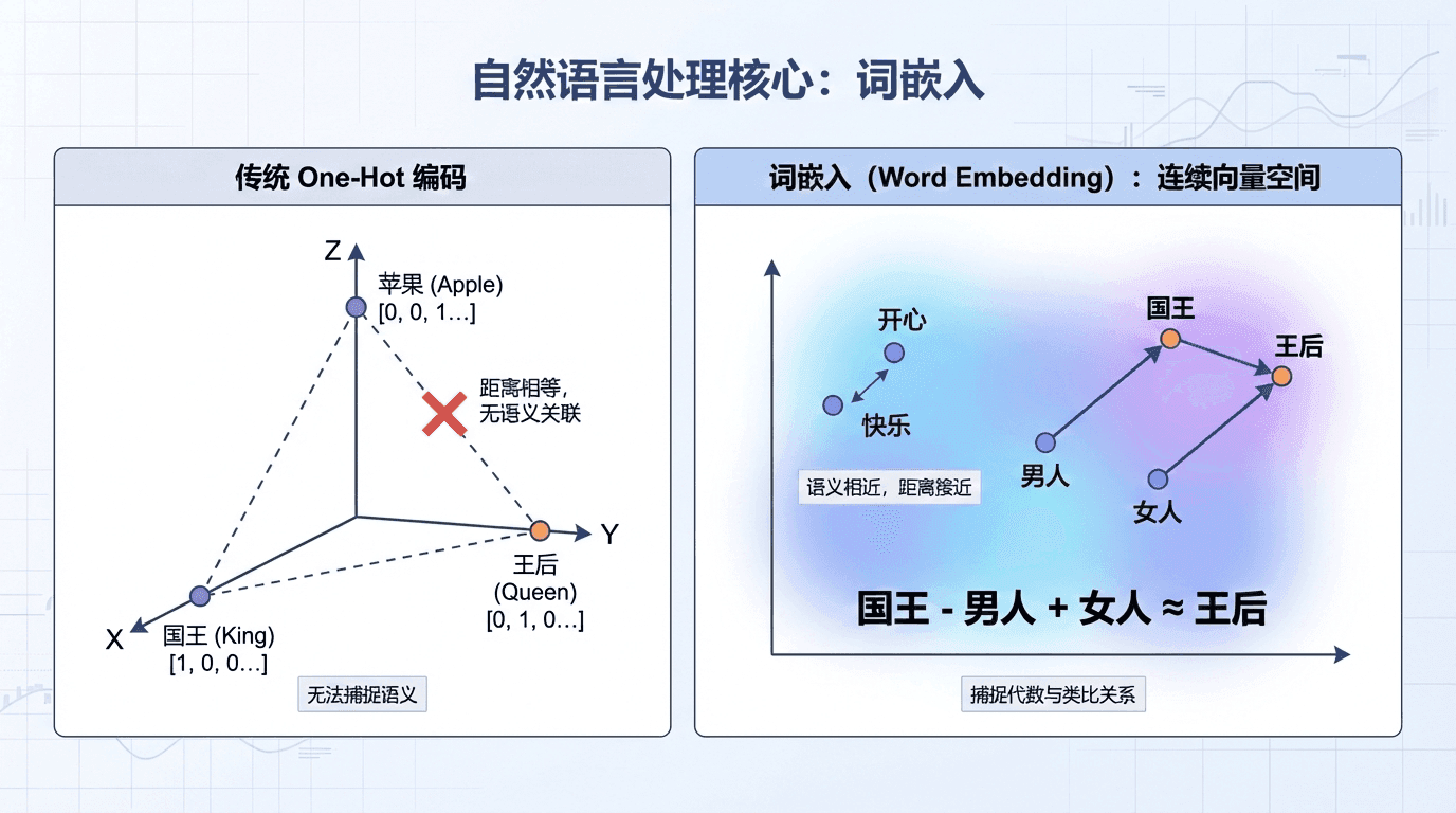
计算机如何理解“国王”和“王后”的关系?如何知道“开心”和“快乐”意思接近?传统的one-hot编码将每个词表示为一个向量,如“国王”是 [1, 0, 0, ..., 0],“王后”是 [0, 1, 0, ..., 0]。这种表示无法捕捉语义——“国王”和“王后”的距离,与“国王”和“苹果”的距离一样远。
词嵌入 (Word Embedding)改变了这一切。它将词映射到连续的向量空间,语义相近的词在空间中距离接近。更神奇的是,词嵌入能捕捉类比关系:“国王” - “男人” + “女人” ≈ “王后”。这种代数结构让机器能理解语言的细微差别。
从One-Hot到嵌入
假设词汇表有10,000个词。One-hot编码将每个词表示为10,000维的稀疏向量,只有一个位置是1其余是0。
问题显而易见:
维度太高 :10,000维,大部分是0,计算和存储浪费无语义信息 :任意两个词的距离都相等(欧氏距离是2 \sqrt{2} 2 泛化能力差 :模型学到"猫很可爱"后,不知道"小猫很可爱"也对
词嵌入将词映射到低维稠密向量,如300维。这300个数字编码了词的各种属性:
注意“国王”和“王后”在性别维度相反,但在皇室维度都很高。这些维度不是人工设计的,而是从数据中学习的。
示例代码:
import numpy as np
# 构建简单的词汇表 vocab = [ '猫' , '狗' , '苹果' , '香蕉' , '喜欢' ] word_to_idx = {word: idx for idx, word in enumerate (vocab)} vocab_size = len (vocab)
def one_hot_encode (word, word_to_idx, vocab_size): """将词转换为one-hot向量""" vector = np.zeros(vocab_size) if word Word2Vec:学习词嵌入
Word2Vec有两种训练方式:Skip-gram和CBOW(Continuous Bag of Words)。
Skip-gram :给定中心词,预测上下文词
输入:“学习”(中心词)
输出:[“我”, “爱”, “深度”, “机器”](上下文词)
数学形式 :
给定词汇表大小 V V V d d d
中心词 c c c o c ∈ R V o_c \in \mathbb{R}^V o c ∈ R V
通过嵌入矩阵 E ∈ R d × V E \in \mathbb{R}^{d \times V} E ∈ R
这里 θ t \theta_t θ t t t t
负采样 优化:
Softmax的分母需要对整个词汇表求和(V=10,000),计算量大。负采样简化为二分类:对于一个正样本(真实的上下文词),随机选K个负样本(不是上下文的词),训练模型区分正负样本。
import numpy as np
def sigmoid (x): """Sigmoid激活函数""" return 1 / ( 1 + np.exp( - x))
# Skip-gram with negative sampling def skipgram_negative_sampling (center_word, context_word, negative_samples, embeddings): """ center_word: 中心词的嵌入,shape (d,) context_word: 上下文词的嵌入,shape (d,) negative_samples: list of negative word embeddings """ # 正样本:中心词和上下文词应该相似 positive_score = sigmoid(np.dot(center_word, context_word)) loss = - GloVe:全局词向量
GloVe(Global Vectors)是另一种流行的词嵌入方法,由Stanford的Pennington等人2014年提出。与Word2Vec不同,GloVe直接利用词的共现统计。
核心思想 :如果词 i i i j j j
J = ∑ i , j = 1 V f ( X i j ) ( w i T w ~ j + b i + b ~ j − log X i j ) 2 J = \sum_{i,j=1}^V f(X_{ij}) (w_i^T \tilde{w}_j + b_i + \tilde{b}_j - \log X_{ij})^2 J = i , j = 1 ∑ V f ( X 这里 X i j X_{ij} X ij i i i j j j f f f
GloVe预训练的词向量(在Wikipedia和Gigaword上训练)可以直接下载使用:
# 加载预训练的GloVe词向量 def load_glove (path = 'glove.6B.100d.txt' ): """加载GloVe词向量""" embeddings = {} with open (path, 'r' , encoding = 'utf-8' ) as f: for line in f: values = line.split() word = values[ 0 ] vector = np.array(values[ 1 :], 词嵌入的类比特性
词嵌入最神奇的性质是能捕捉类比关系。
经典例子:“man” → “woman” 的关系类似于 “king” → ?
数学上,寻找词 w w w
arg max w similarity ( e w , e king − e man + e woman ) \arg\max_w \text{similarity}(e_w, e_{\text{king}} - e_{\text{man}} + e_{\text{woman}}) arg w max similarity ( e w , e king − 用余弦相似度:
similarity ( u , v ) = u T v ∥ u ∥ ∥ v ∥ \text{similarity}(u, v) = \frac{u^T v}{\|u\| \|v\|} similarity ( u , v ) = ∥ u ∥∥ v ∥ u T v 实际测试,答案是“queen”!
其他例子:
“Paris” - “France” + “Japan” ≈ “Tokyo”
“big” - “bigger” + “small” ≈ “smaller”
这种代数结构不是人工设计的,而是从大规模文本中自动学到的。它表明词嵌入捕捉了语言的深层结构。
def cosine_similarity (u, v): """计算余弦相似度""" return np.dot(u, v) / (np.linalg.norm(u) * np.linalg.norm(v))
def analogy (word_a, word_b, word_c, embeddings, top_k = 1 ): """ 完成类比:word_a 对 word_b 的关系,类似于 word_c 对 ? 例如:king - man + woman ≈ queen 返回:最相似的k个词 """ if word_a not in embeddings or word_b not in embeddings or word_c not in embeddings: 实践应用:情感分类
词嵌入最常见的应用是作为NLP模型的输入层。
import torch import torch.nn as nn
# 数据预处理:将文本转换为索引序列 def text_to_indices (text, word_to_idx, max_length = 50 ): """ 将文本转换为词索引序列 text: "这部电影很棒" 返回: [123, 456, 789, 234, 0, 0, ...] # 填充到max_length """ words = text.split() indices = [] for word in words: if word in word_to_idx: indices.append(word_to_idx[word]) else : 使用预训练词嵌入相当于迁移学习——词的语义知识从大规模文本迁移到你的小任务。
词嵌入的偏见问题
词嵌入从真实文本学习,会继承人类的偏见。研究发现:
“doctor” - “man” + “woman” ≈ “nurse”(性别刻板印象)
“程序员”的嵌入向量在性别维度更接近“男性”
这在实际应用中可能导致歧视性结果(如简历筛选系统)。解决方案包括去偏算法、平衡训练数据等,但这仍是研究中的问题。
在最后一节中,我们将学习注意力机制和Seq2Seq模型——机器翻译、文本摘要等任务的核心技术。注意力机制是2017年Transformer革命的基础,理解它对理解现代NLP至关重要。
in
word_to_idx:
vector[word_to_idx[word]] = 1
return vector
# 示例
cat_onehot = one_hot_encode( '猫' , word_to_idx, vocab_size)
dog_onehot = one_hot_encode( '狗' , word_to_idx, vocab_size)
print ( f "'猫'的one-hot编码: { cat_onehot } " )
# 输出: [1. 0. 0. 0. 0.]
print ( f "'狗'的one-hot编码: { dog_onehot } " )
# 输出: [0. 1. 0. 0. 0.]
# 计算距离 - 所有词之间的距离都相等!
from scipy.spatial.distance import euclidean
print ( f "'猫'和'狗'的距离: { euclidean(cat_onehot, dog_onehot) :.2f } " )
print ( f "'猫'和'苹果'的距离: { euclidean(cat_onehot, one_hot_encode( '苹果' , word_to_idx, vocab_size)) :.2f } " )
# 都是 1.41 (sqrt(2))
d × V
e c = E ⋅ o c e_c = E \cdot o_c e c = E ⋅ o c 预测上下文词 t t t p ( t ∣ c ) = e θ t T e c ∑ j = 1 V e θ j T e c p(t | c) = \frac{e^{\theta_t^T e_c}}{\sum_{j=1}^V e^{\theta_j^T e_c}} p ( t ∣ c ) = ∑ j = 1 V e θ j T e c e θ t T e c np.log(positive_score
+
1e-7
)
# 加小值避免log(0)
# 负样本:中心词和负样本应该不相似
for neg_word in negative_samples:
negative_score = sigmoid(np.dot(center_word, neg_word))
loss += - np.log( 1 - negative_score + 1e-7 )
return loss
# 完整的Word2Vec训练示例(简化版)
class Word2Vec :
def __init__ (self, vocab_size, embedding_dim):
self .vocab_size = vocab_size
self .embedding_dim = embedding_dim
# 中心词嵌入和上下文词嵌入
self .W_center = np.random.randn(vocab_size, embedding_dim) * 0.01
self .W_context = np.random.randn(vocab_size, embedding_dim) * 0.01
def train_pair (self, center_idx, context_idx, negative_indices, lr = 0.01 ):
"""训练一个中心词-上下文词对"""
center_vec = self .W_center[center_idx]
context_vec = self .W_context[context_idx]
# 正样本梯度
pos_score = sigmoid(np.dot(center_vec, context_vec))
pos_grad = (pos_score - 1 ) * context_vec
# 更新中心词向量
self .W_center[center_idx] -= lr * pos_grad
# 负样本梯度
for neg_idx in negative_indices:
neg_vec = self .W_context[neg_idx]
neg_score = sigmoid(np.dot(center_vec, neg_vec))
neg_grad = neg_score * neg_vec
self .W_center[center_idx] -= lr * neg_grad
def get_embedding (self, word_idx):
"""获取词的最终嵌入(中心词和上下文词的平均)"""
return ( self .W_center[word_idx] + self .W_context[word_idx]) / 2
# 使用示例
vocab_size = 10000
embedding_dim = 300
model = Word2Vec(vocab_size, embedding_dim)
# 训练:给定句子"我 爱 深度 学习"
# 中心词"爱"(索引1234),上下文词"我"(索引890), "深度"(索引2345)
# 负样本:随机选5个不相关的词
center_idx = 1234
context_idx = 890
negative_indices = [ 100 , 200 , 300 , 400 , 500 ]
model.train_pair(center_idx, context_idx, negative_indices)
ij
)
(
w i T
w ~ j
+
b i +
b ~ j −
log X ij ) 2
dtype
=
'float32'
)
embeddings[word] = vector
return embeddings
glove = load_glove()
# 使用:查找最相似的词
def find_similar_words (word, embeddings, top_k = 5 ):
if word not in embeddings:
return []
word_vec = embeddings[word]
similarities = {}
for other_word, other_vec in embeddings.items():
if other_word != word:
# 余弦相似度
sim = np.dot(word_vec, other_vec) / (np.linalg.norm(word_vec) * np.linalg.norm(other_vec))
similarities[other_word] = sim
return sorted (similarities.items(), key =lambda x: x[ 1 ], reverse = True )[:top_k]
# 示例
print (find_similar_words( 'king' , glove))
# 可能输出:queen, prince, monarch, emperor, ...
e man +
e woman )
return None
# 计算目标向量
target = embeddings[word_a] - embeddings[word_b] + embeddings[word_c]
# 计算所有词与目标向量的相似度
similarities = []
for word, vec in embeddings.items():
# 排除输入的三个词
if word not in [word_a, word_b, word_c]:
sim = cosine_similarity(target, vec)
similarities.append((word, sim))
# 按相似度降序排序
similarities.sort( key =lambda x: x[ 1 ], reverse = True )
if top_k == 1 :
return similarities[ 0 ][ 0 ]
return [(word, sim) for word, sim in similarities[:top_k]]
# 使用示例
print ( "类比测试:" )
print ( f "man:woman :: king:? => { analogy( 'man' , 'woman' , 'king' , glove) } " )
# 输出: queen
print ( f "big:bigger :: small:? => { analogy( 'big' , 'bigger' , 'small' , glove) } " )
# 输出: smaller
print ( f "Paris:France :: Tokyo:? => { analogy( 'Paris' , 'France' , 'Tokyo' , glove) } " )
# 输出: Japan
# 返回top-3结果
print ( " \n 更详细的结果(top-3):" )
results = analogy( 'man' , 'woman' , 'king' , glove, top_k = 3 )
for word, similarity in results:
print ( f " { word } : { similarity :.3f } " )
# 可能输出:
# queen: 0.856
# monarch: 0.721
# princess: 0.698
indices.append(word_to_idx[ '<UNK>' ]) # 未知词
# 填充或截断到固定长度
if len (indices) < max_length:
indices += [word_to_idx[ '<PAD>' ]] * (max_length - len (indices))
else :
indices = indices[:max_length]
return indices
# 简单的情感分类模型
class SentimentClassifier ( nn . Module ):
def __init__ (self, vocab_size, embedding_dim, hidden_dim):
super (). __init__ ()
self .embedding = nn.Embedding(vocab_size, embedding_dim, padding_idx = 0 )
self .rnn = nn.LSTM(embedding_dim, hidden_dim, batch_first = True )
self .fc = nn.Linear(hidden_dim, 2 ) # 正面/负面
def forward (self, x):
# x: (batch_size, seq_length) 词索引序列
embedded = self .embedding(x) # (batch, seq, emb_dim)
_, (h_n, _) = self .rnn(embedded) # h_n: (1, batch, hidden)
output = self .fc(h_n.squeeze( 0 )) # (batch, 2)
return output
# 使用预训练的GloVe初始化embedding层
def load_glove_matrix (word_to_idx, glove_path = 'glove.6B.300d.txt' , embedding_dim = 300 ):
"""加载预训练GloVe向量,构建嵌入矩阵"""
vocab_size = len (word_to_idx)
embedding_matrix = np.zeros((vocab_size, embedding_dim))
# 读取GloVe文件
glove_dict = {}
with open (glove_path, 'r' , encoding = 'utf-8' ) as f:
for line in f:
values = line.split()
word = values[ 0 ]
vector = np.array(values[ 1 :], dtype = 'float32' )
glove_dict[word] = vector
# 为词汇表中的每个词赋值
found = 0
for word, idx in word_to_idx.items():
if word in glove_dict:
embedding_matrix[idx] = glove_dict[word]
found += 1
else :
# 随机初始化未找到的词
embedding_matrix[idx] = np.random.randn(embedding_dim) * 0.01
print ( f "在GloVe中找到 { found } / { vocab_size } 个词" )
return embedding_matrix
# 创建模型并加载预训练嵌入
vocab_size = 10000
embedding_dim = 300
hidden_dim = 128
model = SentimentClassifier(vocab_size, embedding_dim, hidden_dim)
# 加载预训练嵌入
pretrained_embeddings = load_glove_matrix(word_to_idx)
model.embedding.weight.data.copy_(torch.from_numpy(pretrained_embeddings))
# 选择1:冻结embedding层(数据很少时)
model.embedding.weight.requires_grad = False
# 选择2:微调embedding层(数据较多时)
# model.embedding.weight.requires_grad = True
# 训练示例
texts = [ "这部电影很棒" , "太失望了" ]
labels = [ 1 , 0 ] # 1=正面, 0=负面
# 转换为索引
inputs = torch.tensor([text_to_indices(text, word_to_idx) for text in texts])
targets = torch.tensor(labels)
# 前向传播
outputs = model(inputs)
print ( f "模型输出: { outputs } " )
print ( f "预测类别: { torch.argmax(outputs, dim = 1 ) } " )